One of SatDump’s major components is projections. Geo-referencing satellite data, especially when it’s not in GEO requires quite a few convoluted processing steps.
Considering one recent set of changes involved greatly improving the entire projection system’s internals, I thought it would be a good idea to do a little article explaining the entire process in details, especially since this not something I have seen documented in any “simpler” way when I was doing research at the time.
Part of a FengYun-3F DPT Dump, projected MERSI-3
So how exactly, do we get there?
Special thanks to Digielektro for the implementation I borrowed for quite a while and Fred Jansen for the advice.
Note : The implementations / processes described here concern the “reworked” version now in use after 1.1.0
Where’s the instrument pointing?
This might seem trivial for us looking on the imagery, it’s pretty obvious where land is… But obviously, we can’t rely on that, therefore we instead need to calculate it purely from the information either provided by the satellite in the data or external information such as TLEs.
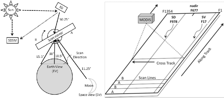
First of all though, it may be a good idea to introduce how most imaging/sounding instruments scan in the first place. Taking the example of an instrument often seen as a reference, the AVHRR (NOAA and MetOp’s imager) the concept is quite simple. It’s a telescope, rotating 5 times per second and taking a sample (pixel) of each line 2048 times while it’s looking down. This process keeps going as the satellite moves forward in reference to the ground, and the instrument scanning (very) “roughly” orthogonal to the satellite’s direction, this results in the image being built up this way, slowly.
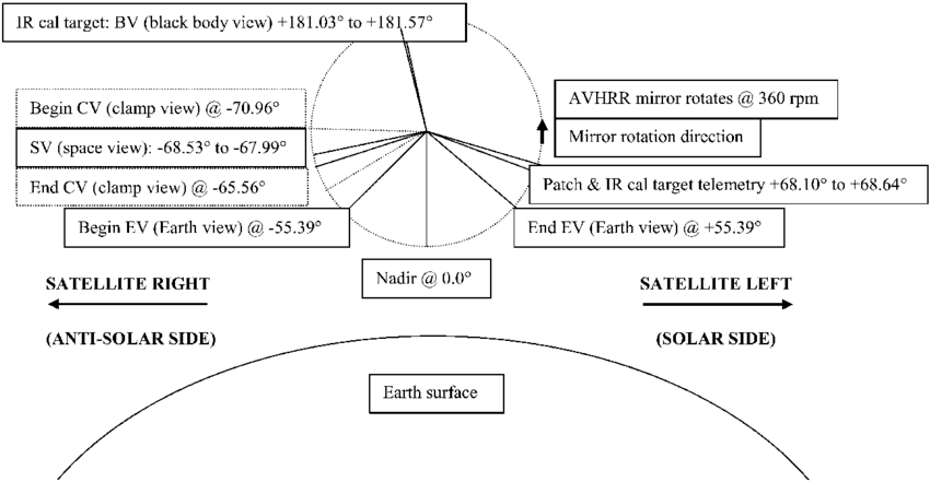
In this diagram, pictured is a more detailed version of the cycle AVHRR performs every rotation. This includes calibration readings and more, but here this doesn’t matter, just note that most similar instruments follow a very similar method.
The one thing of interest for later however is “Nadir”. This is a very common term which simply refers to the point right below the satellite, toward the center of Earth (or rather, the WGS84 ellipsoid used to model the Earth’s shape).
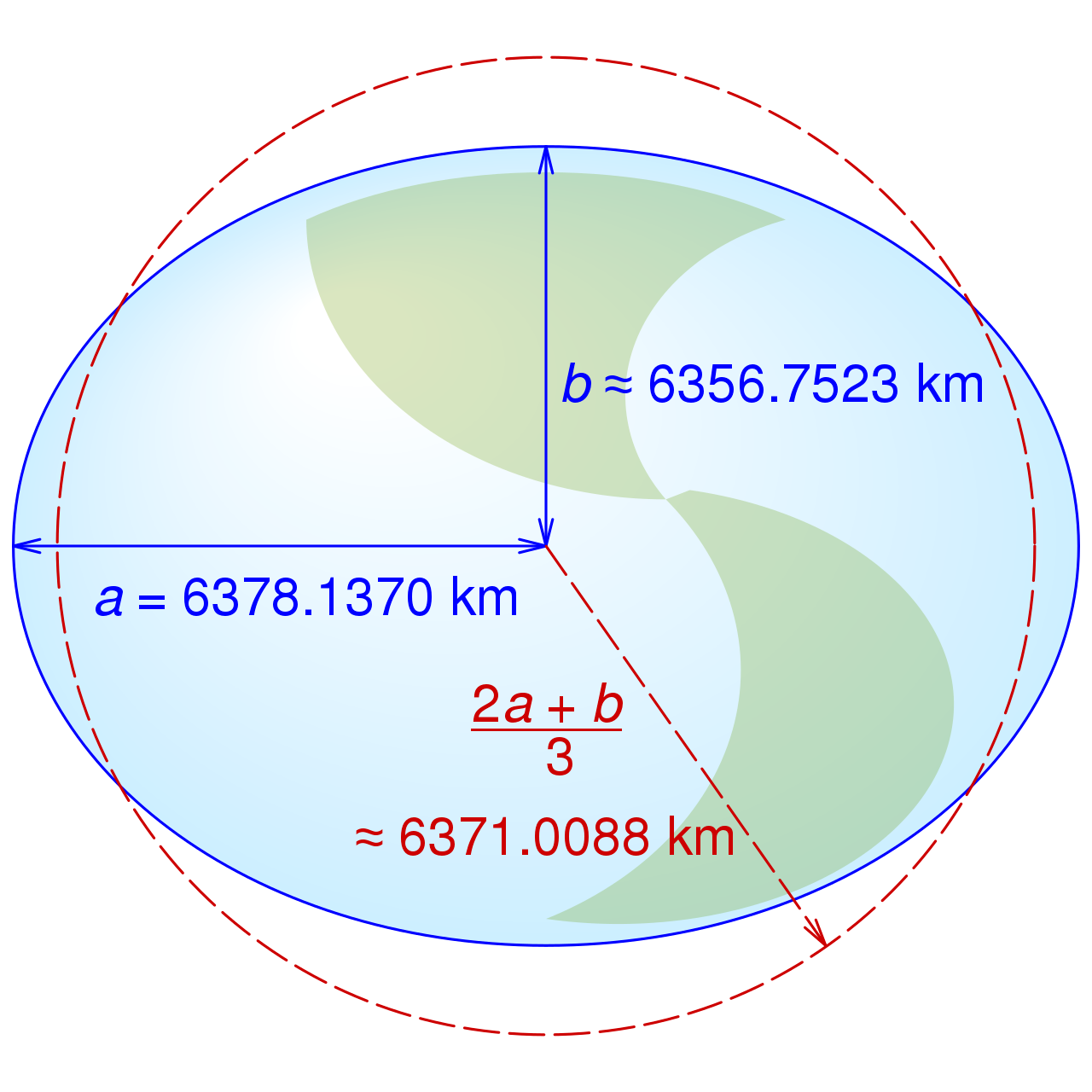
This WGS84 represents a good approximation of the Earth’s surface, but ignoring more specific topology (eg, oceans, land, mountains, etc), which are too small to care about anyway with what we’re doing here. It is usually navigated with “LLA” geodetic (Latitude, Longitude, Altitude) coordinates with altitude = 0 being on the surface of the model. However, for some of the other required operations it is necessary to work in cartesian (X, Y, Z) coordinates instead. In that case, since we’re working with the Earth as a reference, they will be in ECI with the center of the WGS84 ellipsoid as 0, 0, 0.
Now that we’ve got the base concepts, the first issue is knowing where the satellite was located as a certain scan was being done. This is usually done by simply putting a timestamp within the telemetry, referencing the scanline’s time. This timestamp may be a bit offset, such that is actually is a bit before/after the start of the scan, but they provide a good reference nonetheless.
Given a timestamp, it is then possible to run the SGP4 model using TLEs (yes, the same used to control rotators and know when the satellite’s passing) and calculate very accurate state vectors of the satellite. State vectors are composed of the satellite’s position in meters and cartesian x/y/z coordinates and the velocity vector (where the satellite’s going) in meters per second.
Then… While we now know where the satellite is and where it’s going, that’s not enough. We also have to know how it is positioned in orbit. That’s called the attitude of the spacecraft, however we’ll need to make a few more assumptions. First of all, we will assume the spacecraft always points to (or rather, is stable relative to) Nadir, which is a reasonable assumptions to make for most missions carrying such imagers. Secondly, we will assume it is stable relative to the velocity vector (which also happens to follow Nadir, as we’re orbitting Earth). That’s also a fair assumption to make for nearly all concerned missions.
From there, we have a reference assuming the spacecraft is perfectly aligned but that in reality is not the case. Furthermore instruments mounted on the satellite itself may not be so perfectly and have some added offset. Finally, the instrument scans around, pointing at what can be expressed as an offset relative to the (assumed) S/C position.
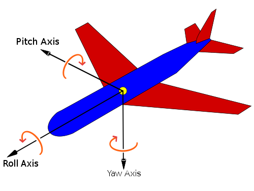
So to summarize, instrument pointing can be expressed as angles relative the roll axis (which is the velocity vector), the yaw axis (nadir vector, or pointing straigth down) and pitch axis which is a vector orthogonal to the velocity (roll) vector. With those angles, an instrument look vector pointing down to Earth can be built by consecutive rotations.
But first, how do we generate the Nadir vector? It is not provided by SGP4 like the velocity vector is, however we can simply switch between coordinate systems : SGP4 position coordinates are in cartesian, but can be converted to geodetic (LLA). Altitude is now relative to the center of the WGS84 model, so setting it to 0 will put it right on the Earth’s surface. We can then convert back to cartesian coordinates and calculate the vector between those two positions.
Now that we have the two necessary vectors, any attitude offsets can be applied in a few rotations :
- Apply yaw by rotating the velocity vector around the nadir vector
- Generate another vector, let’s call it
p, which is a rotation by 90 degrees of the velocity vector - Apply roll by rotating the nadir vector around the velocity vector
- Apply pitch by rotating the nadir vector around
p - We now have a vector representing instrument pointing towards Earth
After this, we need to calculate where this vector actually intersects with Earth. Here, I’m using some math implemented by Digielektro (from the algorithm I had previously borrowed before this new revision, why rewrite it if it works?).
1
2
3
4
5
6
7
8
9
10
11
12
13
14
15
16
const double &a = geodetic::WGS84::a;
const double &b = geodetic::WGS84::a;
const double &c = geodetic::WGS84::b;

double value = -pow(a, 2) * pow(b, 2) * w * position.z - pow(a, 2) * pow(c, 2) * v * position.y - pow(b, 2) * pow(c, 2) * u * position.x;
double radical = pow(a, 2) * pow(b, 2) * pow(w, 2) + pow(a, 2) * pow(c, 2) * pow(v, 2) - pow(a, 2) * pow(v, 2) * pow(position.z, 2) +
                 2 * pow(a, 2) * v * w * position.y * position.z - pow(a, 2) * pow(w, 2) * pow(position.y, 2) + pow(b, 2) * pow(c, 2) * pow(u, 2) -
                 pow(b, 2) * pow(u, 2) * pow(position.z, 2) + 2 * pow(b, 2) * u * w * position.x * position.z - pow(b, 2) * pow(w, 2) * pow(position.x, 2) -
                 pow(c, 2) * pow(u, 2) * pow(position.y, 2) + 2 * pow(c, 2) * u * v * position.x * position.y - pow(c, 2) * pow(v, 2) * pow(position.x, 2);
double magnitude = pow(a, 2) * pow(b, 2) * pow(w, 2) + pow(a, 2) * pow(c, 2) * pow(v, 2) + pow(b, 2) * pow(c, 2) * pow(u, 2);

double d = (value - a * b * c * sqrt(radical)) / magnitude;

position.x += d * u;
position.y += d * v;
position.z += d * w;
This method basically “scales” the pointing vector to be the exact magnitude (or, “length”), which can be added to the spacecraft’s position to get the cartesian coordinates of the intercept, and converted to latitude and longitude.
From there, we need to calculate yaw, pitch, roll angles for each instrument’s pixel (sample). Most of them rotate around roll and take a sample at a regular (angular) interval which makes it really simple to calculate. Static offsets can then be applied to correct for instrument mounting (eg, the center pixel may not actually be pointing down perfectly), but also to correct for the fact the satellite keeps moving during the scan, which result in it appearing slightly at an angle compared to the surface (that is corrected by applying a yaw offset).
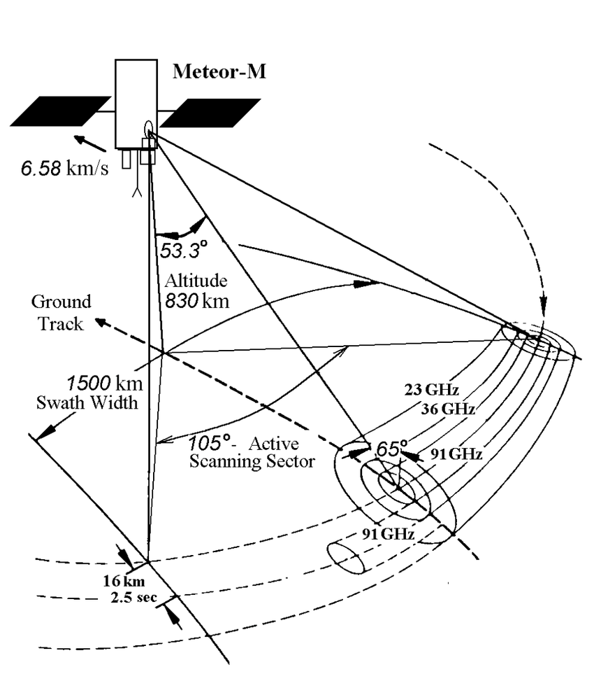
Some instruments, say MTVZA or MWRI rotate around yaw while pointing “forward”. The same idea applies otherwise, just a different axis.
And now, given all this it is possible to calculate the Earth location of any pixel by :
- Getting the timestamp for the current scan
- Calculating the satellite position with SGP4
- Calculating instrument pointing for the current pixel
- Raytrace it to Earth
- Convert to Geodetic coordinates
But now, how do we use this information to project the image on another map?
The case of warps
The next problem in line may seem trivial at first… And trust me with that, I thought so at first! Let me explain.
We have the ability to calculate the relation from the satellite image to Earth. But if we do something simple, that is just calculate the position and plot it on a map for each pixel, well, there’s an issue : what do we do for the points… In between!? Long ago I solve this problem with a stupid algorithm that just draw a big, fat circle around that position to “make it look mostly ok”. Might have worked, but that’s an awful solution.
The right approach is actually to do the opposite : for each pixel of the target projection, calculate which pixel corresponds on the raw image. However, while it is definitely not impossible, this would get extremely convoluted mathematically. So we can actually take a big shortcut : Thin-Plate-Spline Interpolation.
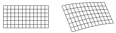
As seen above, this is an algorithm which given a few reference points between 2 planes to interpolate (approximate) the transformation between those 2. This means that instead of complicated inverse math, we can calculate a few reference points and easily get a transformation (the math to convert between) the raw image and its projection on Earth’s surface.
I initially wrote my own implementation, but ended up borrowing The GDAL Project’s which was far more optimized. I have also ported it over to OpenCL, which allows running it on the GPU with far greater performance, since the operation can easily be extremeley parralelized and ported to rely on single-precision (32-bits) floats which graphics card excell at crunching through. That results in easily over 10x faster processing than a CPU, taking at most seconds versus minutes :-).
Either way, this is pretty much it for the “normal” operation of re-projecting…
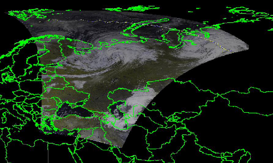
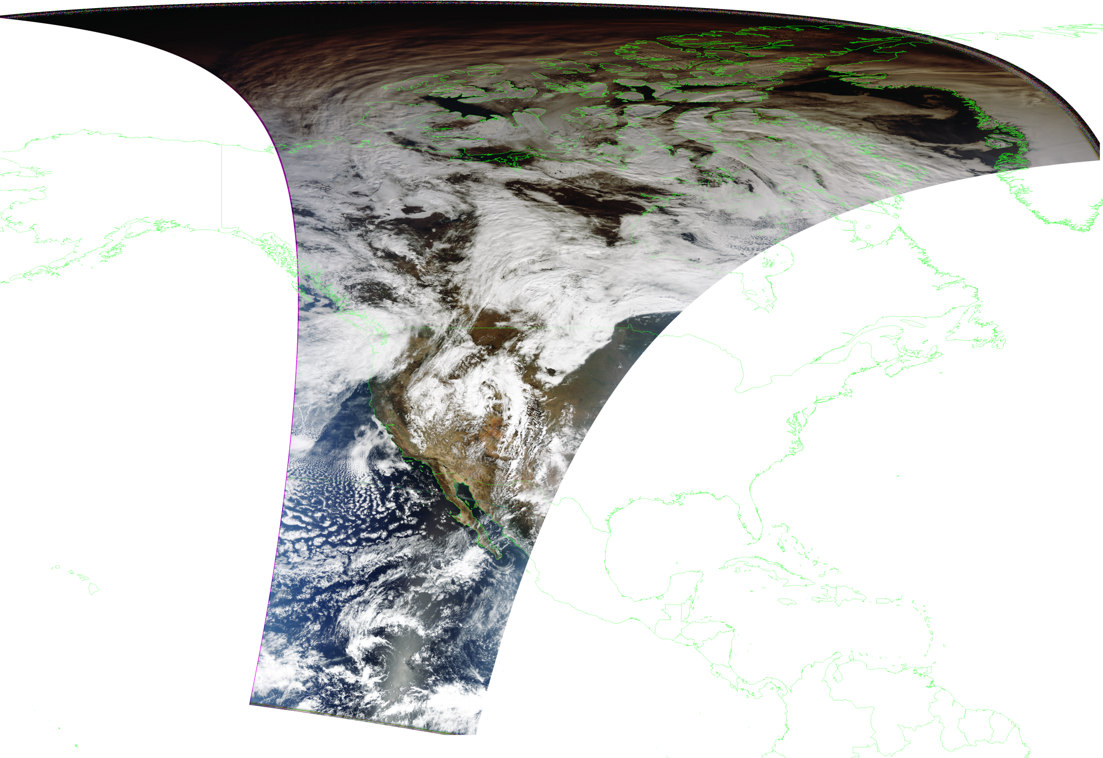
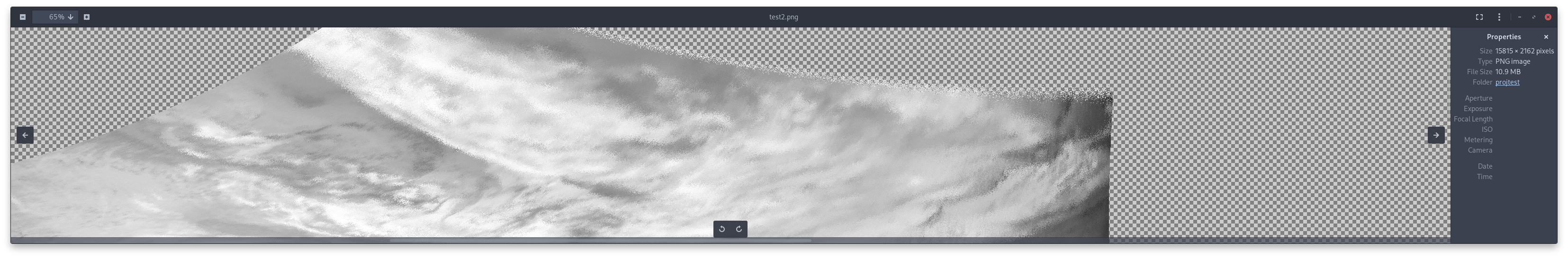
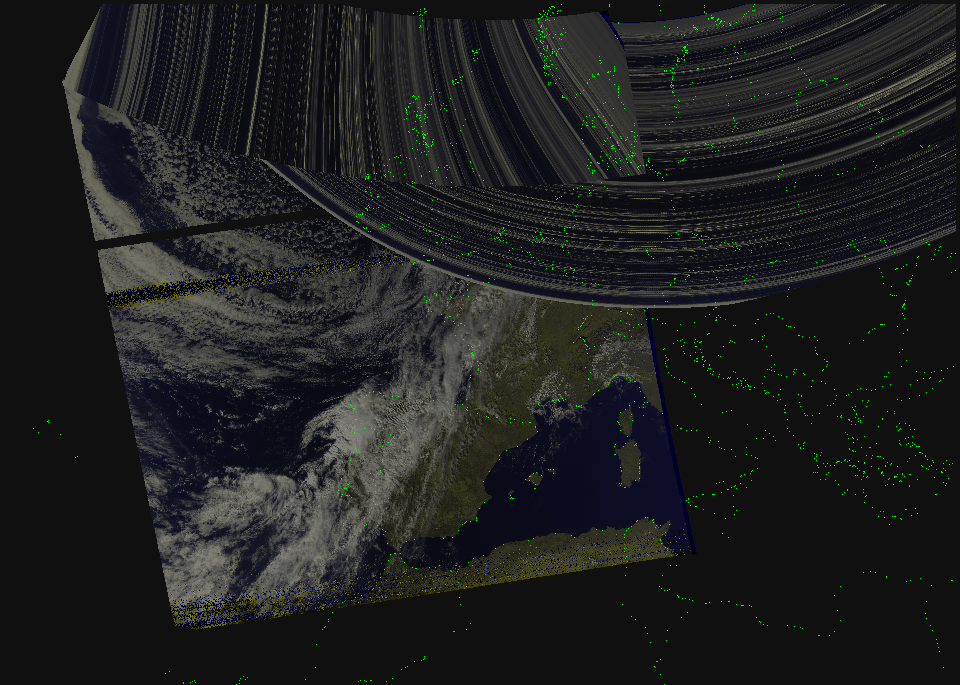
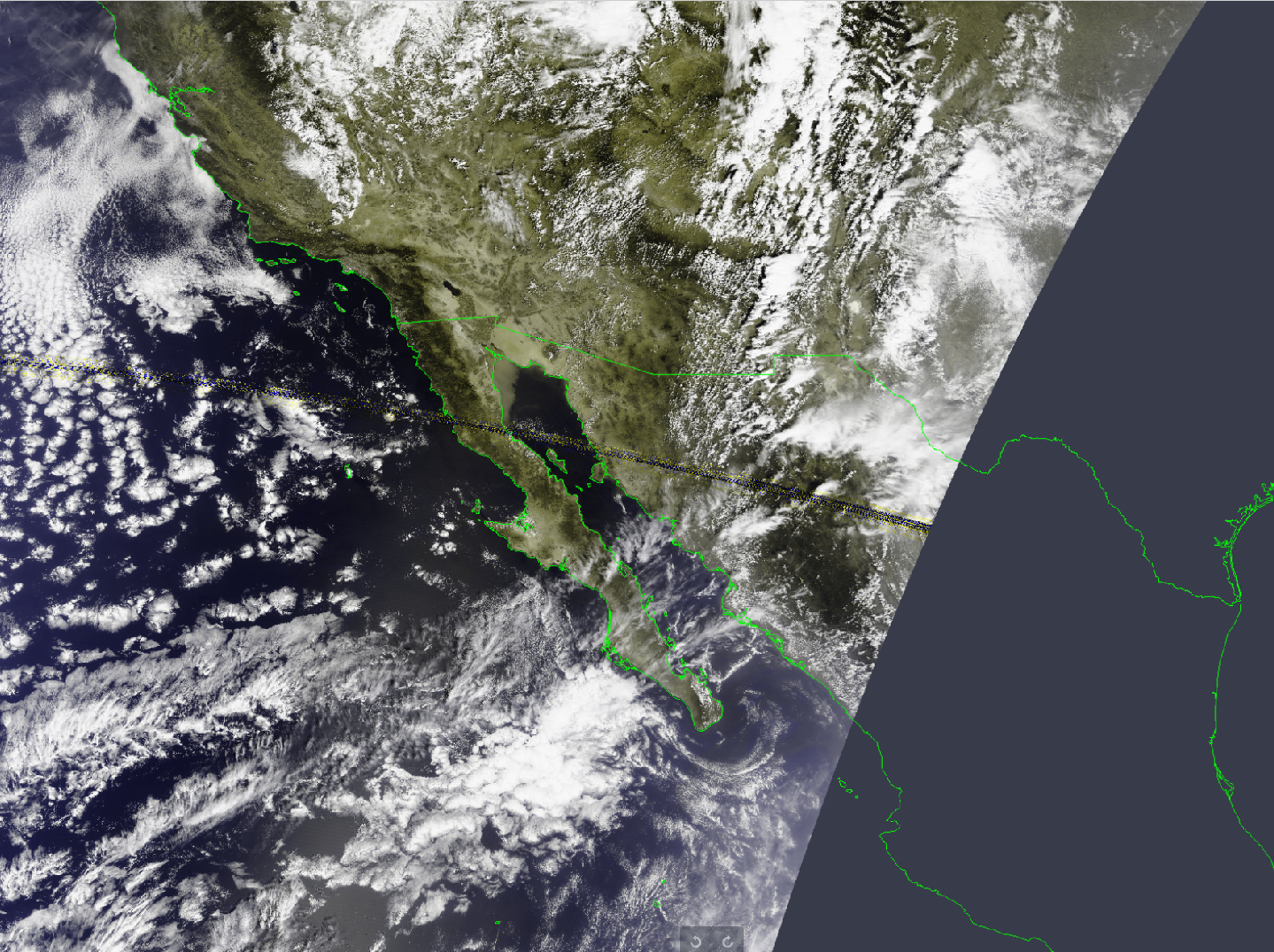
However, there are a few problems with this approach that will only occur in specific cases : when you’re either cross the south or north pole, or when “rolling over” in longitude… And it makes sense! It’s working on a plane, it has no idea we’re actually on a sphere… So when crossing borders, it just goes wrong and can result in a variety of artefacts, especially on dumps such as NOAA GAC.
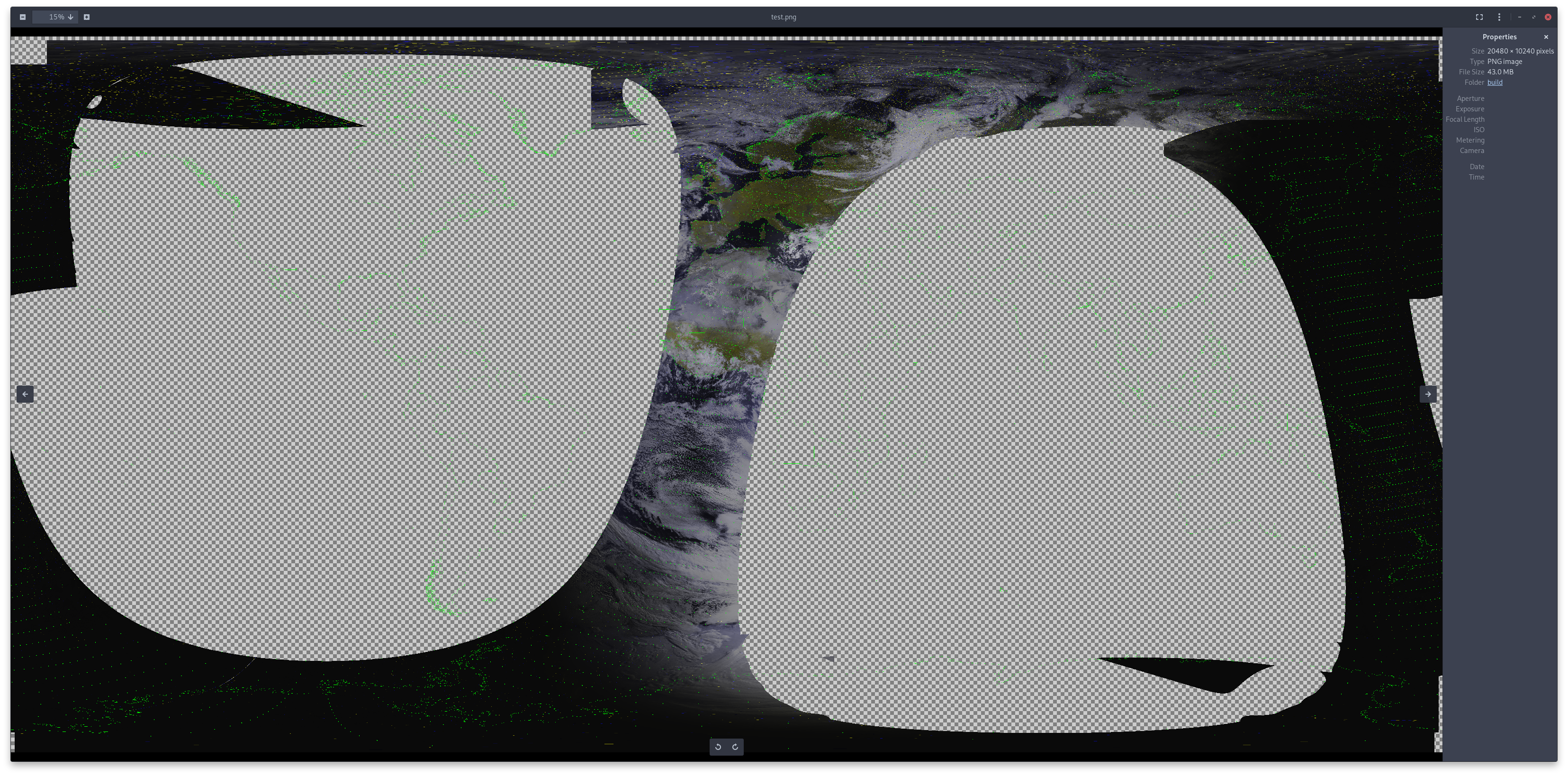
As you can see on this image, it overall looks pretty good - except there are a few random chunks spread around that do not below there at all (the green dots are the reference points)! This is in fact, one of the unexpected behavior that happened when nothing is done to keep the plane the TPS (interpolation) continuous.
So, what do we do? In reality the idea is pretty simple : Shift everything so it’s in the center, never crossing any border.
In longitude this is very simple, it simply consist of applying an offset to bring it around 0. Hence the procedure is rather simple :
- Get all the reference points and calculate their mean longitude
- Apply the inverse offset to bring them all toward 0, 0 on the points being given to the interpolation algorithm
- Apply the same offset when requesting a point
Doing it this way, on the points and before going through the TPS function keeps it entirely transparent to the rest of the algorithm, except it doesn’t break :-) Hence at this point, projecting a dump (without the poles) works exactly as expected!
But now, what about the poles? You would likely be tempted to apply the same method as we did with longitude, but it’s not that simple. Rather, why not exploit the fact the Earth is round? (Sorry, flat earthers)
Instead of simply offseting toward the center, we can apply a spherical rotation toward the pole (to basically make it “as if” the north/south pole were at the center of the map). However this is a bit more involved.
1
2
3
4
5
6
7
8
9
10
11
12
13
14
15
16
17
18
19
void shift_latlon_by_lat(double *lat, double *lon, double shift)
{
    if (shift == 0)
        return;

    double x = cos(*lat * DEG_TO_RAD) * cos(*lon * DEG_TO_RAD);
    double y = cos(*lat * DEG_TO_RAD) * sin(*lon * DEG_TO_RAD);
    double z = sin(*lat * DEG_TO_RAD);

    double theta = shift * DEG_TO_RAD;

    double x2 = x * cos(theta) + z * sin(theta);
    double y2 = y;
    double z2 = z * cos(theta) - x * sin(theta);

    *lon = atan2(y2, x2) * RAD_TO_DEG;
    double hyp = sqrt(x2 * x2 + y2 * y2);
    *lat = atan2(z2, hyp) * RAD_TO_DEG;
}
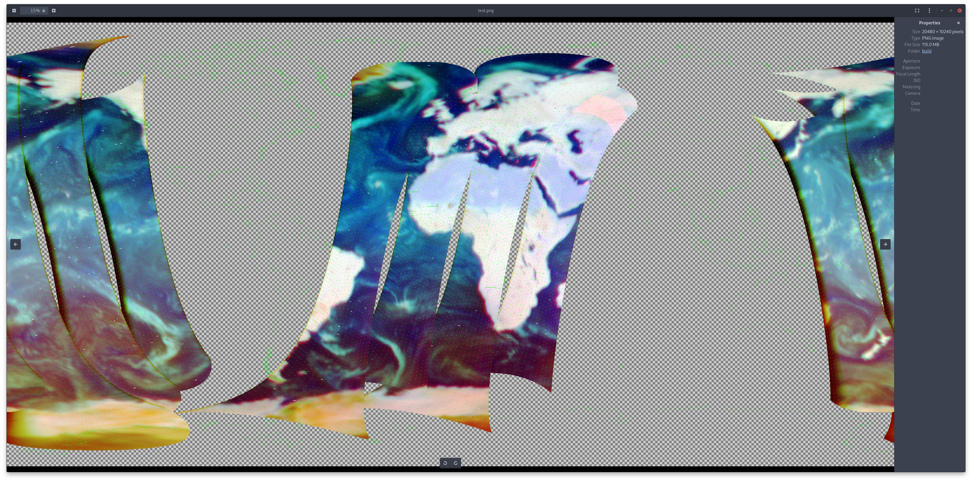
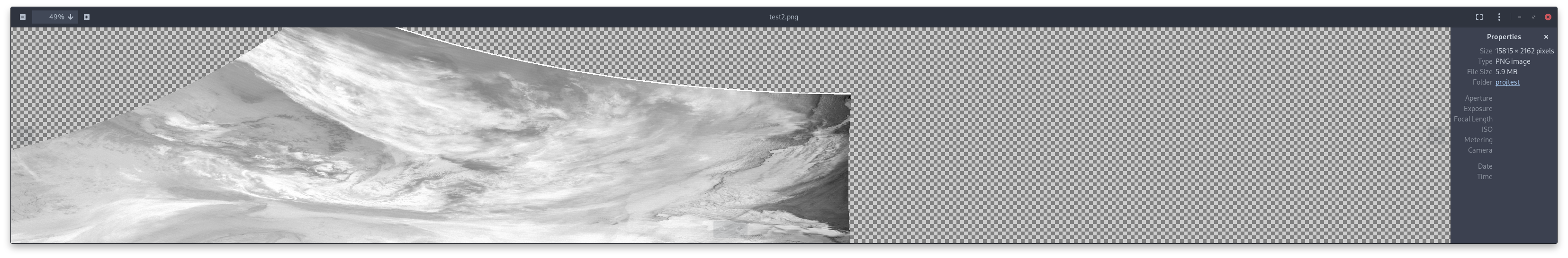
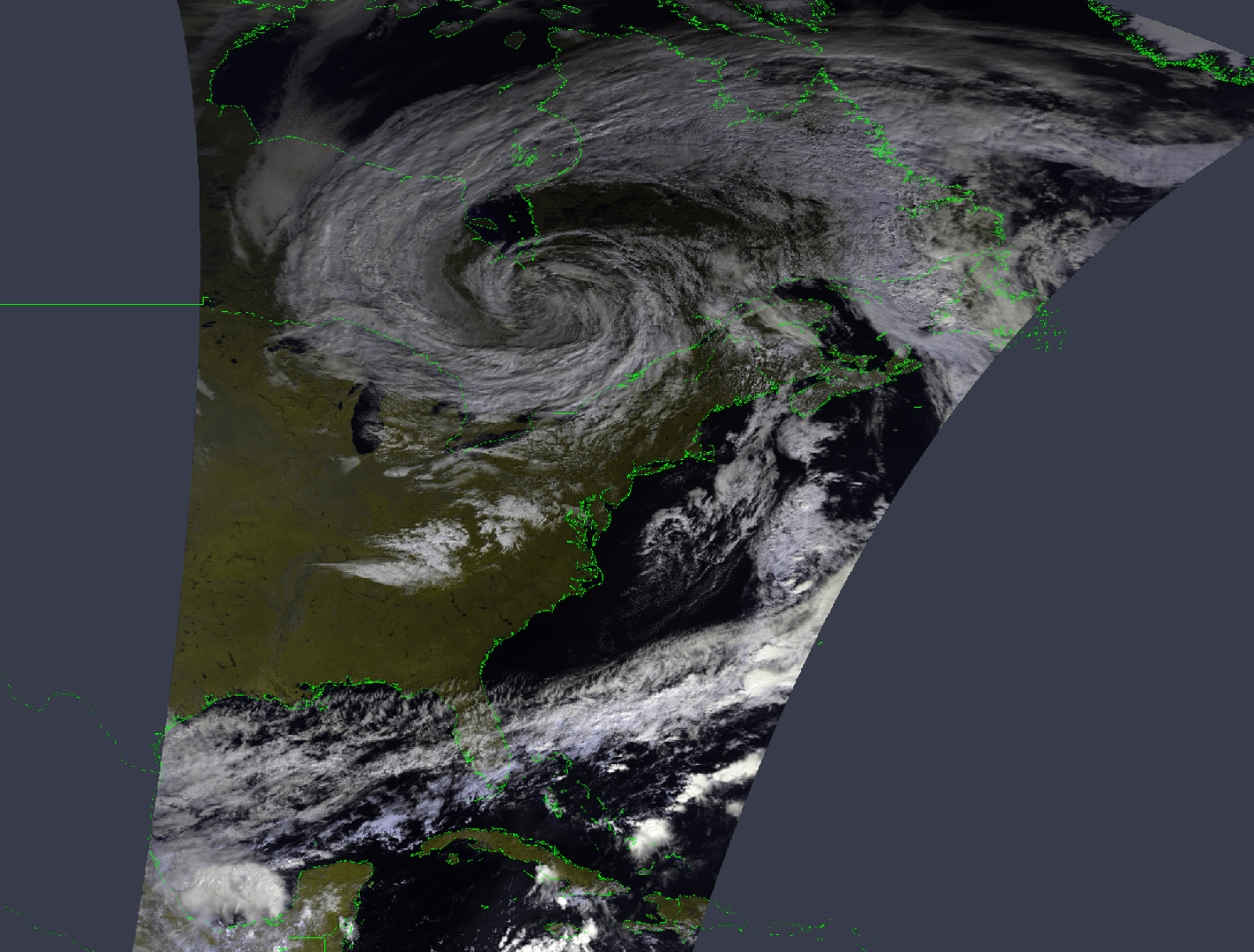
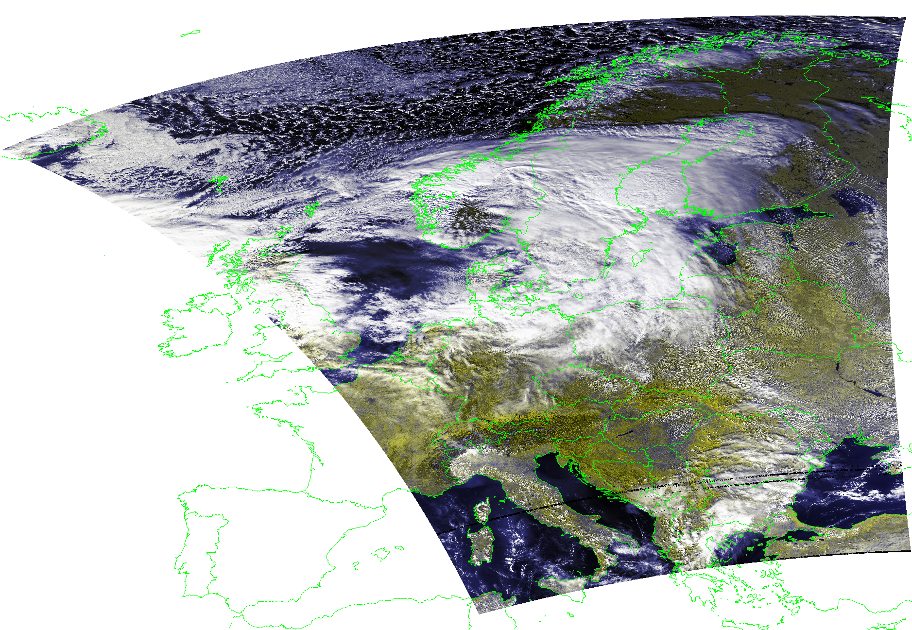
The idea is basically to convert every geodetic coordinate being provided to cartesian, and rotating it around 0, 0, 0, then back to cartesian. This produces (internally), the following result, just ignore the artefacts on the map.
As you can see now, evidently, anything near the pole will now not be cut in any way, and rather appear like any other normal pass!
After implementating that fix in the same way as the longitude one, the TPS algorithm now never gets any “cut” plane to work with, which fixes those issues entirely.
Finally, a last detail for dumps is… They have to be split into many “small segments”. This is not the hardest part, it’s some basic math to calculate how long they are and ensure they never exceed the length of a normal “Direct Broadcast” pass. This just consists of calculating the average distance between points along the y axis of the image, approximating the “kilometers” covered and splitting according to that.
Deeper into the weeds
Above, I covered mainly the processes utilized, glancing over the nicher stuff as not to make it too confusing straight away - but in this part I will guide you through some of the… Less fun occurences stumbled upon during development.
Double Precision… Wait no?
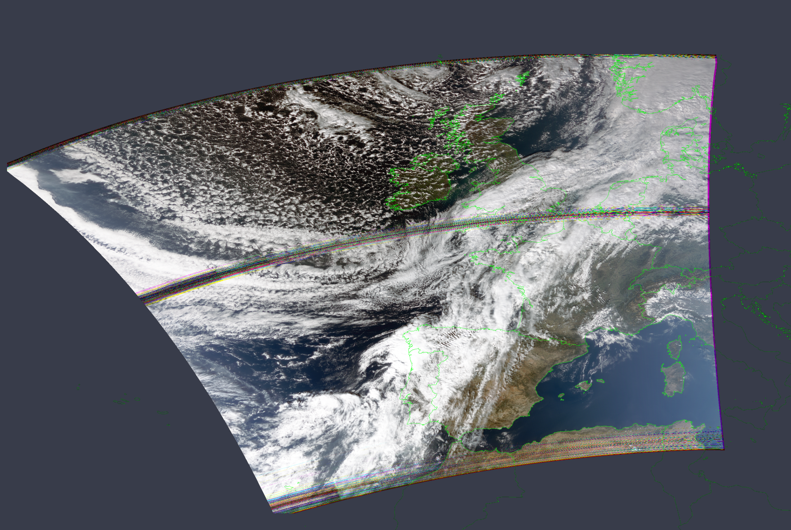
For quite a while, after fixing the pole issue I was being reported a worrying behaviour. The image would just get… Fuzzy!?
My first reaction was that the latitude rotation/shift was causing an issue, so I removed it and… Nothing!? So, as a first effort to begin debugging, I disabled GPU processing as to test on the CPU, and… It worked fine!?
At this point I had absolutely no clue, so I started playing around and at some point realized one major difference. The CPU version is written exclusively using double, while the “normal/fast” GPU version uses exclusively float. Why does that matter though? double is 64-bits, while float is 32, so float is far less precise… And can’t go as high/lower in the values it can hold. I therefore tired a last-ditch effort switching the GPU code to double (there is disabled version in SatDump already), and… Go figure, it also worked flawlessly. I then proceeded to waste a good 5 hours debugging without any success.
I had given up and basically forced double when covering the poles to fix the issue, but this is around when I switched to the instrument raytracing method described above (from Digielektro’s matrix-based/Azimuth-based approach). That magically fixed this “fuzziness” issue somehow! I’m not entirely sure and I have not felt like digging into why, but my intuition is that the previous ray-tracking algorithm was getting too imprecise over the poles, causing bad control points to be generated and messing with the TPS interpolation. The double version hence likely was able to overcome those parasites while float simply lacked the precision required to do so.
MetOp - Or sheer luck
For the longest time using Digielektro’s approach, MetOp was the only satellite to actually get any sort of reliably accurate projections for some reasons. I knew this implementation had issues, but… It worked “OK” with MetOp.
However, when I switched everything over the new (proper) approach described earlier…
I figured I had messed up the configuration or such… But… No. The offset was way off on the other side?
From there, I had no idea. I shortly thought it was maybe a maneuver on MetOp, so I tried more data with the same disastrous results… After doing some research though, it turns out it is indeed MetOp’s fault! EUMETSAT has decided to make them steer around the yaw axis to correct for the Earth’s rotation and other things. Not sure why, but OK.
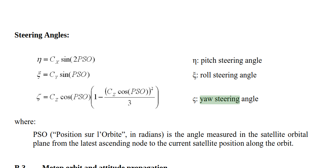
I haven’t yet implementated this alongside the new approach, but how incredible is it that a bug in one implementation just happens to counter MetOp’s unusual attitude-keeping scheme? I still have a hard time believing it… However it does make some sense, at the old algorithm was ignoring a bunch of other factors.
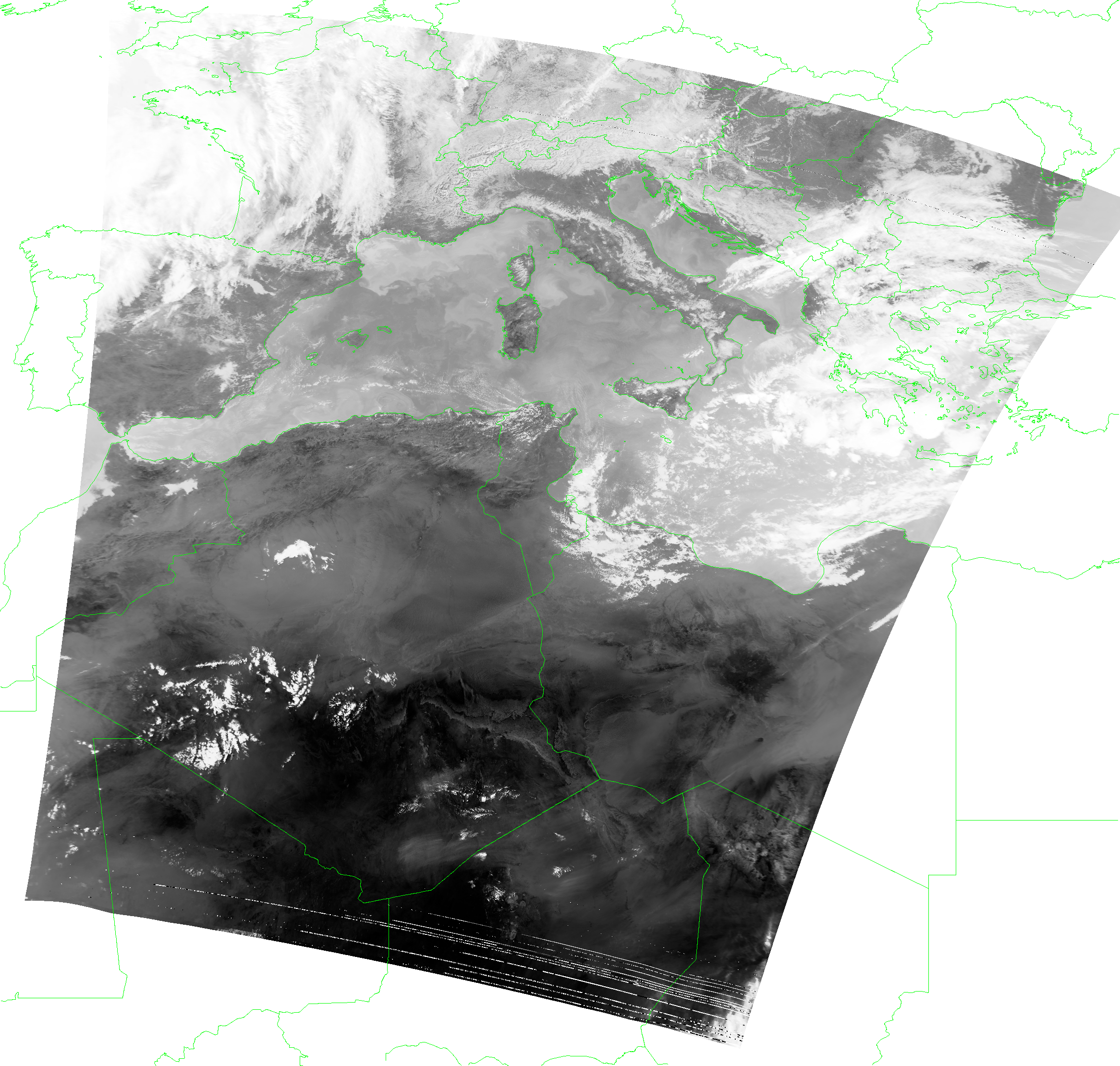
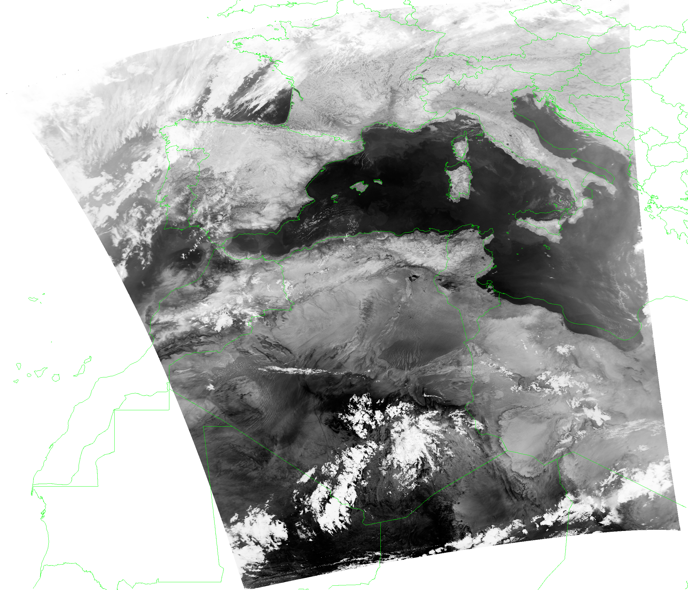
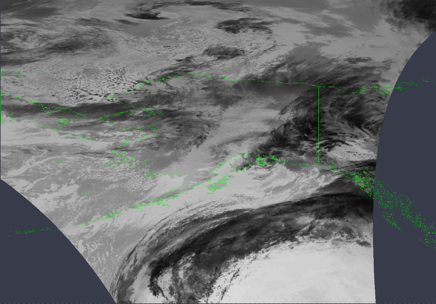
Corrupted Timestamps
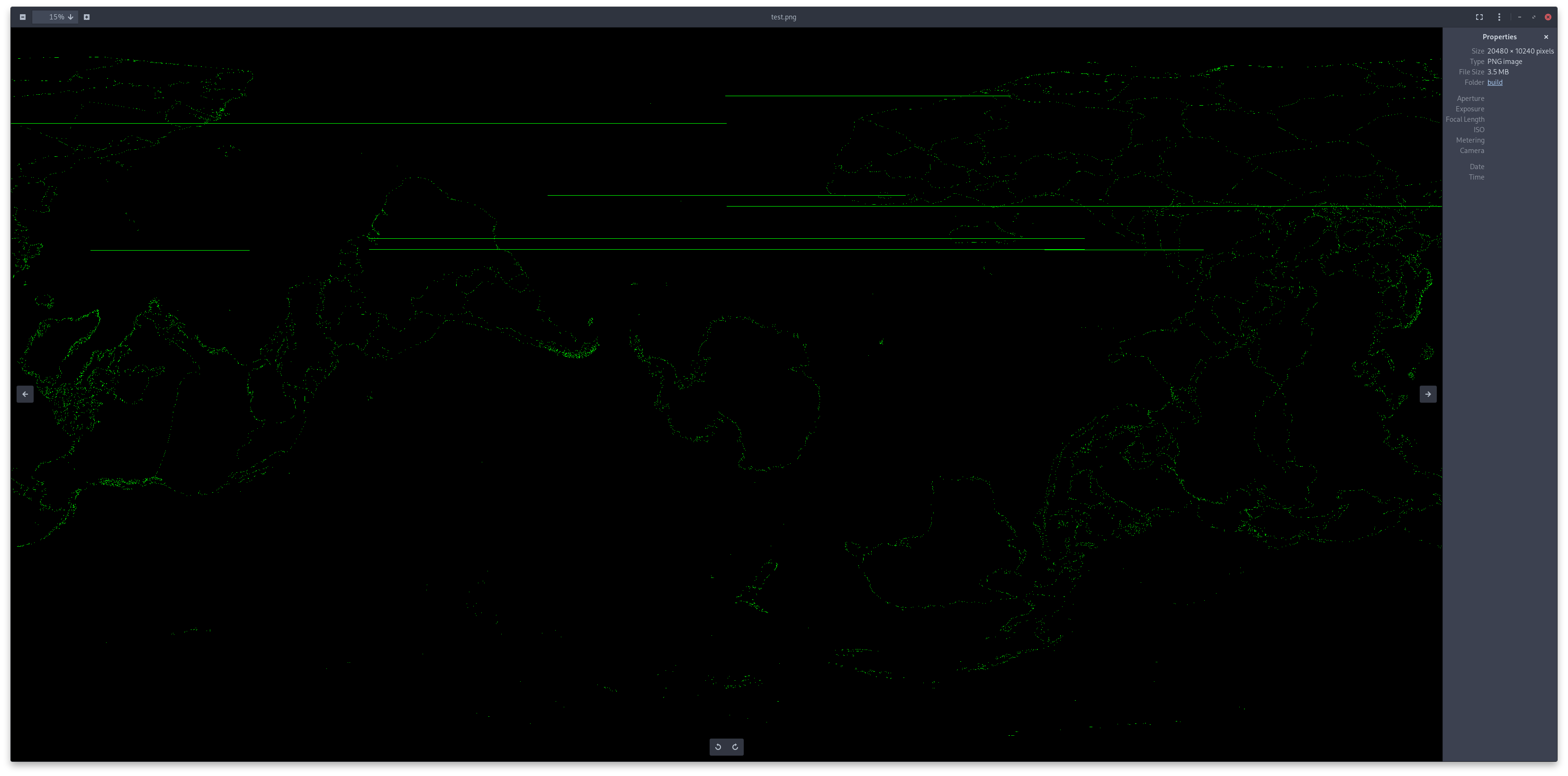
As stated previous, most instruments provide timestamp that are mandatory for the rest of the processing toward projections. However, quite often a file can contain corrupted timestamps that need to be filtered out. This is done with an algorithm written a while back, which does some basic statistics-based filtering. It’s rather simple but has been performing rather very well as of now. Further processing can also be done to filter the points themselves instead, which may catch a few more errors. Without such filtering working, you can get this type of results…!
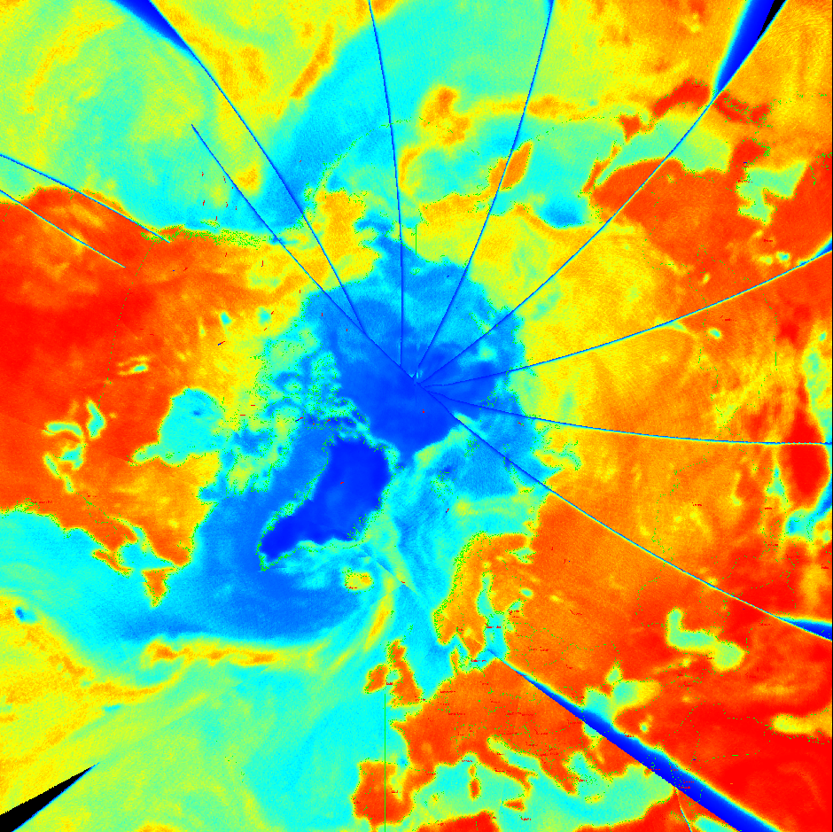
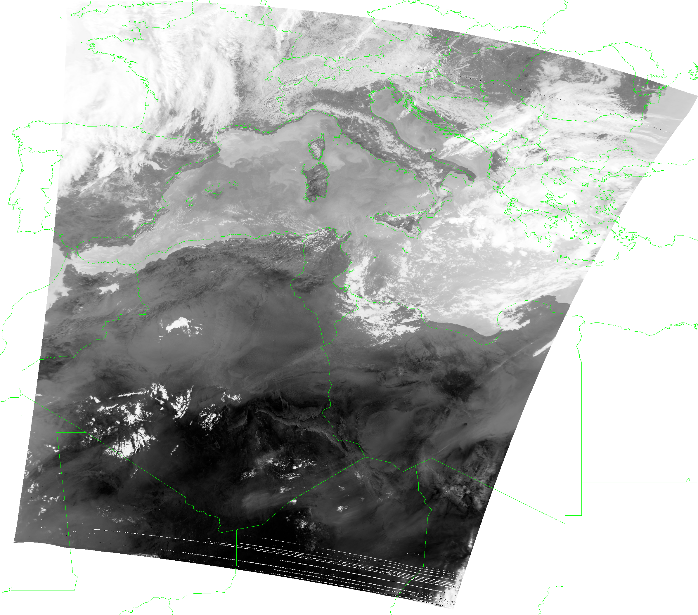
Some results
NOAA-18 by JVital2013
FengYun-3E DPT by Andrew (MrFentazis)
FengYun-3F DPT by Andrew (MrFentazis)
Aqua DB
FengYun-3D AHRPT by Fred Jansen
In conclusion, after quite a bit of long-due work projections are now much more accurate - and enough for good “X-Band-grade” results - with a bunch of other fixes :-)
And of course in case you encounter any issues… Please report.