We’ve noticed that the UI after the rework (even though we think is pretty clean) can be quite confusing to many people. That’s why I’ve have decided to write this post in which I explain some basic features of SatDump and how to use them efficiently!
UI
First Start
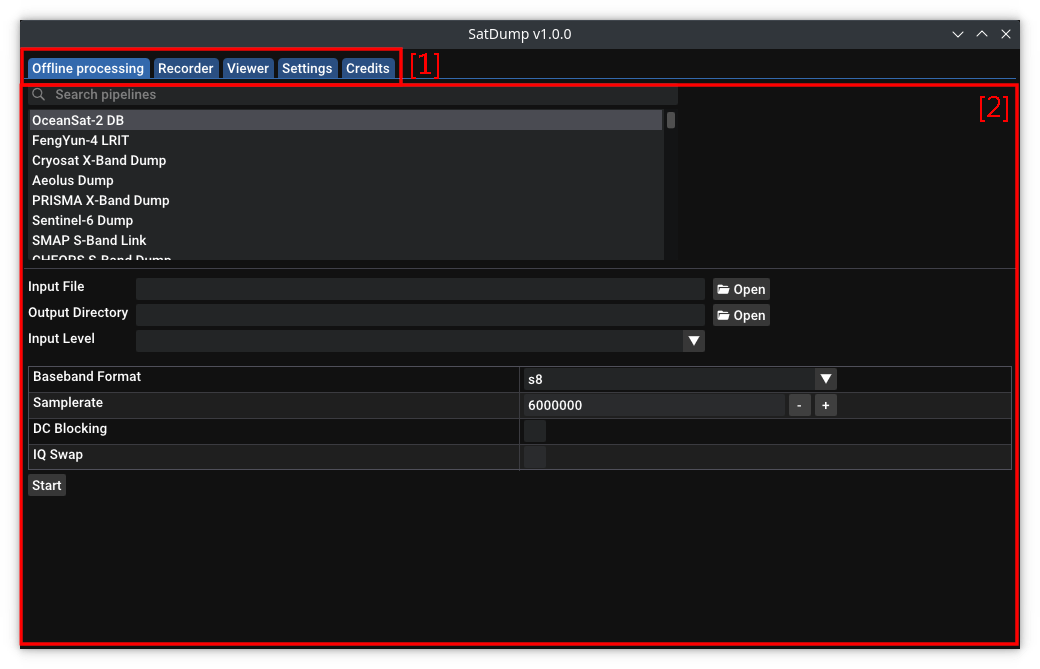
When you launch satdump-ui you are greeted with a GUI window. The main way of navigating in it is the Tab Bar on the top [1]. Using that you can switch between the different tools SatDump has to offer. The UI of each tool is loaded into the main screen [2].
Offline Decoding
This tool (as the name suggests) lets you process data from a file. It can be any level (meaning you can process a baseband as well as a cadu file). the UI can be divided into 3 main sections:
- Pipeline Selection [1]
- File Selection [2]
- Pipeline Options [3]
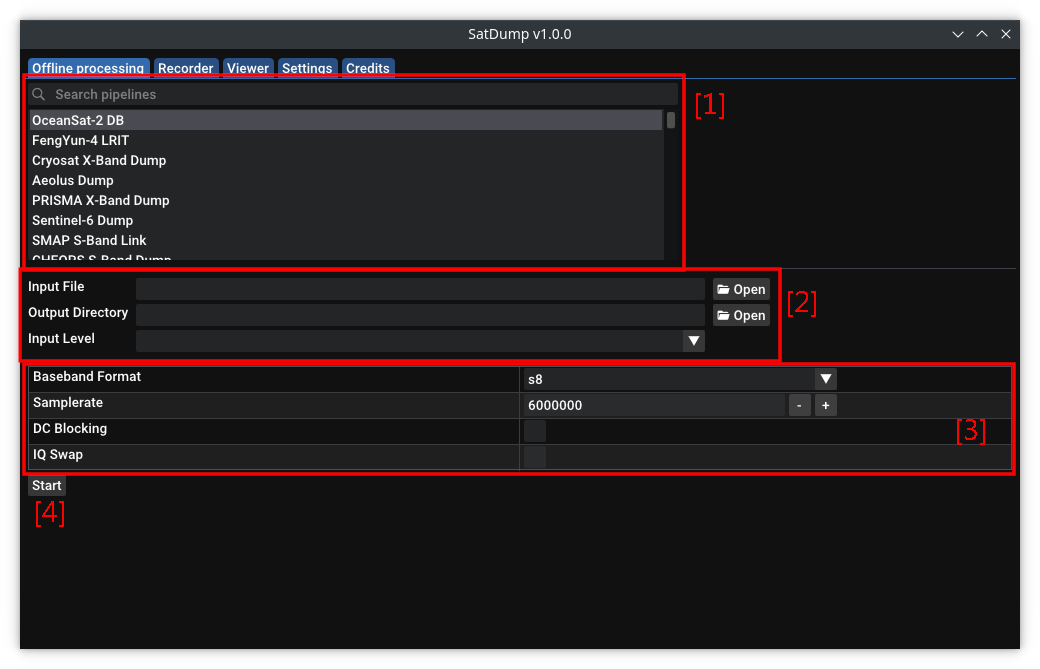
Pipeline Selection
This widgets lets you select which pipeline to use. Each pipeline is specific to one downlink, so for NOAA you have several: DSB, HRPT and GAC.
File Selection
Here you select the input file, output directory as well as input level. While the last may sound complex, it’s really simple. It just specifies what the input file is. Usually baseband is selected when you want to process a recorded signal and cadu or frames (depending on the downlink) is used when processing data coming from live decoding.
Pipeline Options
This table has all the options specific to a pipeline, such as samplerate and baseband format (only valid when you are using baseband as input, otherwise irrelevant).
Once everything is set to the correct values you can start the decoding using the ‘Start’ button [4].
Recorder (Live Processing)
This is new! In this menu, you can find everything that’s related to using an SDR in SatDump. Here you can view, record as well as process data from a radio. Here is the breakdown of the UI:
- Source Controls [1]
- FFT Options [2]
- Processing [3]
- Recording [4]
- FFT and Waterfall [5]
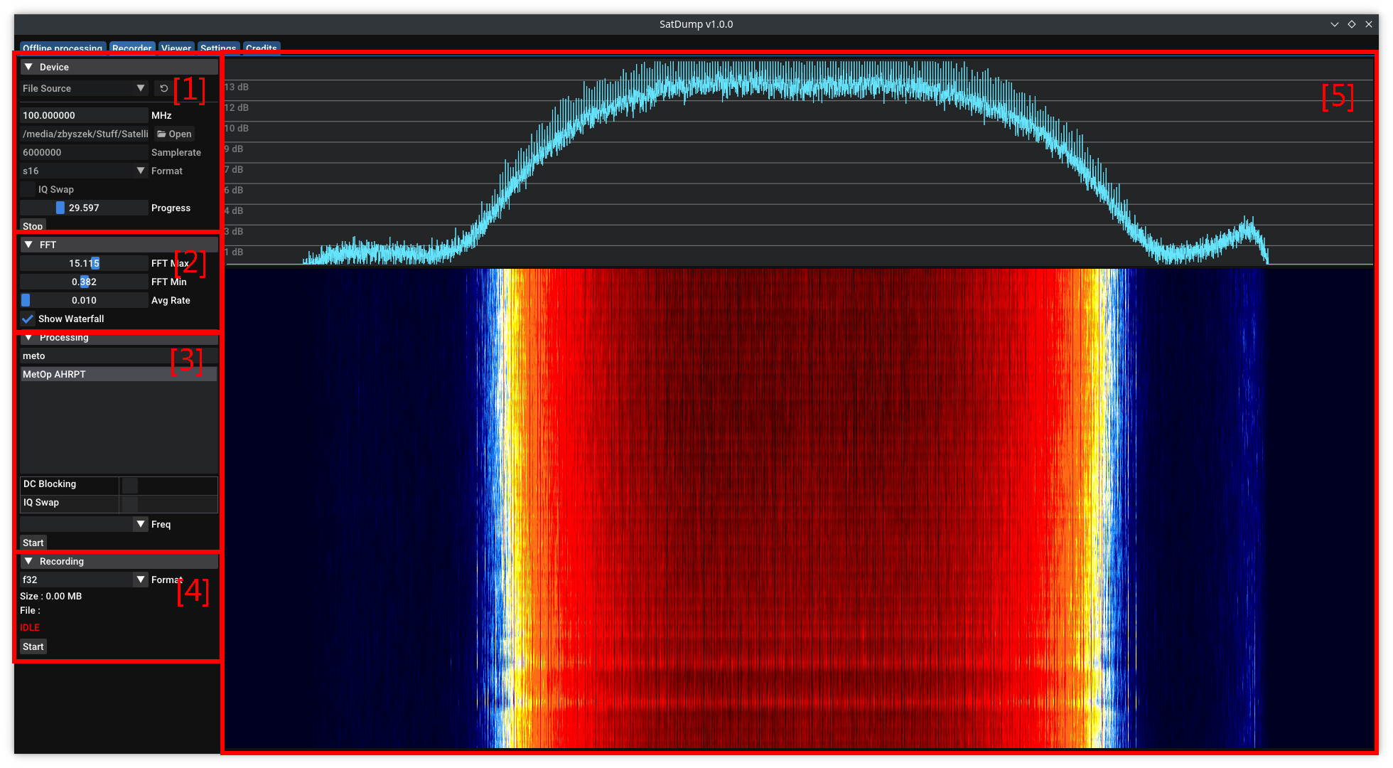
Source Controls
This menu lets you select what source to use (SDR or a file) and has all the options regarding the selected source. Here you set the frequency, samplerate, gain, etc. The menu changes depending on the source. You can refresh the source list by pressing the ‘arrow’ button on the right of the combobox.
FFT Options
Here you can control the FFT and waterfall displays. Using the sliders you can change the displayed range. The sliders change the lower and upper cutoff (so the difference between these is the displayed range). You may also notice the ‘Avg Rate’ slider. This controls the level of averaging applied to the FFT. Lower values give a smoother FFT.
Processing
In this menu you can initiate live decoding. It is simillar in a way to the Offline Decoding section. You can find a pipeline selector and pipeline options in both of them. You may start the processing with the ‘Start’ button. Some new widgets will appear. The output will be saved in a directory specified in the Settings!
Recording
This is a menu where you can Record a baseband file. You have to select a baseband format. available formats are s8 (8 bit), s16 (16 bit), f32 (32bit float), wav16 (wav compatible with other software like SDR++) and ZIQ (custom format using ZSTD compression. Can be added with a CMAKE flag on compilation). Status of the recording is indicated by the colored text.
FFT and Waterfall
This is self explanatory, it’s the FFT and waterfall of the current signal. However it is worth nothing that the waterfall is somewhat intensive! If your PC/Device appears to be struggling/dropping, this may help quite a bit!
The Viewer
This is probably the biggest new feature in SatDump after the rewrite. This menu lets you view, tune and project your data. There are two main tools you can change between using the tabs: Products and Projections. There is too many options to fit into one screenshot so I will have to divide them into several.
Products (Viewer)
Here you can edit and view your decoded images. There are a few menus that house different settings:
- General
- Image
- RGB Composites
- Products
- Map Overlay
- Projection
General
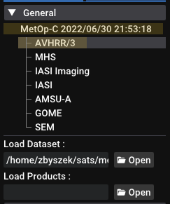
In this menu are the most basic functions. There is a tree view of opened datasets and products and options for laoding new datasets and products. (products are automatically loaded after decoding) When you open the viewer with no products loaded you will be greeted with only this tab and loading options. Note: the product and dataset names are highlighted yellow when they are added to the projection list, more on that later. You can close datasets and products using an x buttonon the right of the name (it can be hidden if the panel is small).
Image
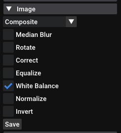
Here you can choose what channel (or composite) to use. You can also apply options such as equalization, white balance, etc. The ‘Save’ button saves the displayed image.
RGB Composites
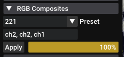
This section gives you controll over the RGB composites. You can select from available presets, but also manually create composites of your liking. To do that, simply enter the formula into the textbox. Satdump will understand basic mathematical and logic (ternary) operators, so you can create more elaborate composites, such as the VIS/IR blend:
ch1 < 0.065 ? (ch4 - 0.7) * 2.66 : ch2 * 2.2 - 0.15, ch1 < 0.065 ? (ch4 - 0.7) * 2.66 : ch2 * 2.2 - 0.15, ch1 < 0.065 ? (ch4 - 0.7) * 2.66 : ch1 * 2.2 - 0.15
Products
This Tab will contain information about calibration and other higher level products we introduce. So far very few instruments are calibrated.
Map Overlay
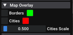
This is where you can choose to overlay your image with a map and/or add city labels. You can change the colors as well as the size of the labels.
Projection
This menu lets you add the data to a projection list. If the data is added it will be indicated with a yellow highlight in the tree view. The ‘Old Algorithm” checkbox lets you select a second projection algorithm for this data. It can be better for projecting bad quality data. It is selected by default on systems that do not support OpenCL (for speed reasons. OpenCL = Graphics Card Computing for short).
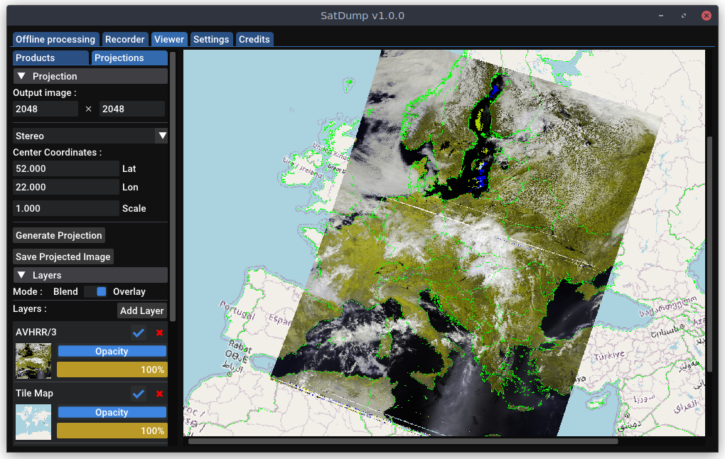
Projections (Viewer)
Here you will find yet another new menu. It controls the projection tool, which lets you apply projections to your data. You can also load backgrounds such as the tile map or images in equirectangular projection. You may find 4 main parts here:
- Projection Menu [1]
- Layers Menu [2]
- Map Overlay Menu [3]
- The Image View [4]
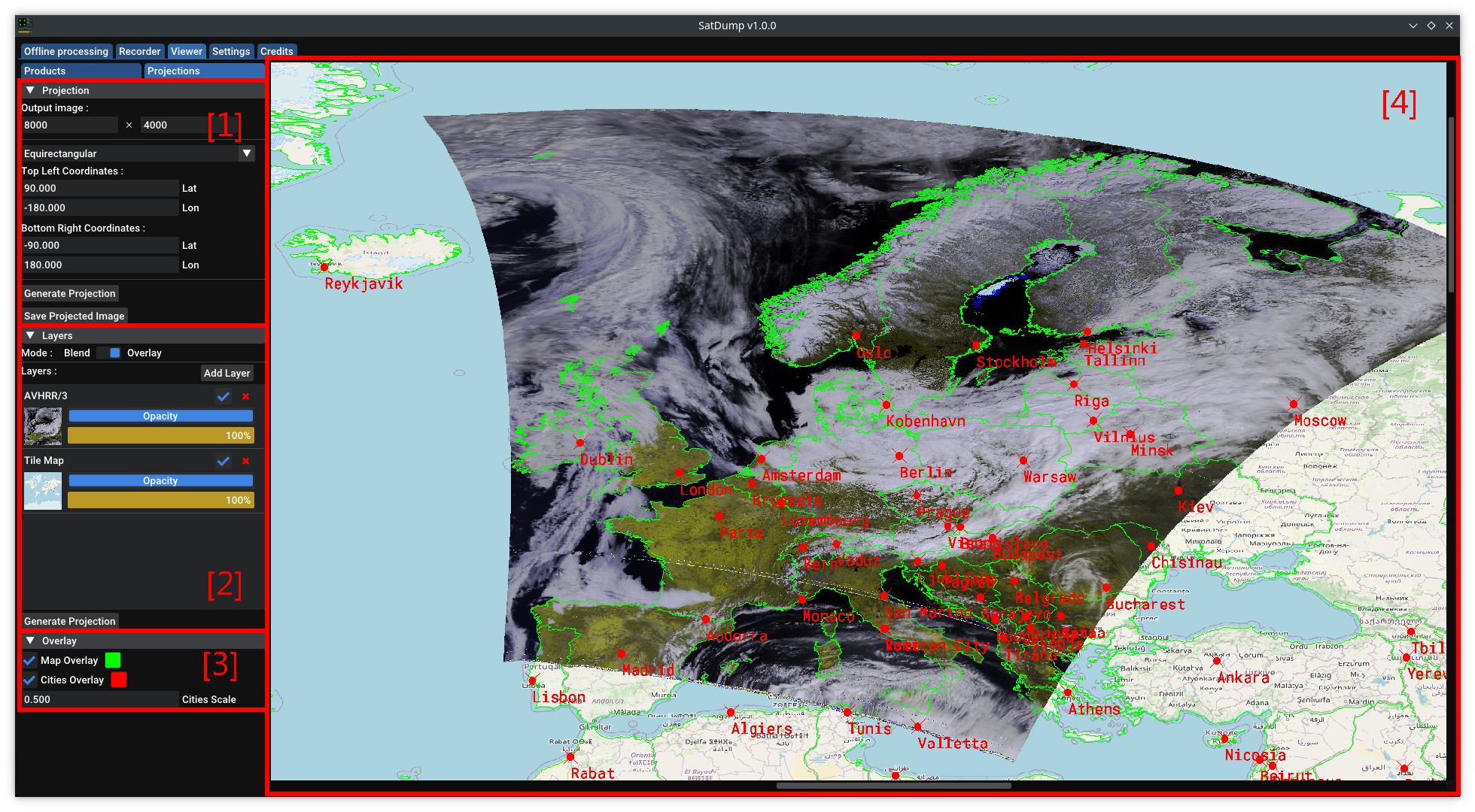
Projection Menu
This is the heart of this whole tool. It houses all the projection settings. In the first line you can select the output image size. Under that you select the target projection. You can use any of the ones listed! Available projections are Equirectangular, Stereographic, Mercator and TPERS. Note: do not use 90 degree latitude in TPERS, it will break! (use something like 89.999) Every projection has its own settings which are displayed under the selection. On the bottom of the menu are two buttons, which you can use to render and save the projected image.
Layers Menu
This is the part I am (personally) most excited about. We have implemented a layer system for the projections. This means you can combine multiple passes into one image easily! On the very top is a mode selector. You can choose between blend and overlay. I tihnk these are self explanatory!
Under that the layer list is located. There is an Add Layer button on the left. This will bring you to a separate window where you can laod custom layers such as Tile Maps, equirectangular images and gesotationary satellite images. You can load basically any image if you provide it with an appropriate configuration file (more on that in another post, TODO). As proof that you can load anything here is an Obama Sphere.
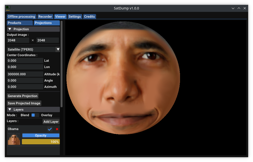
Lastly there is the star of the show: the layer list! Each layer has a thumbnail, an enable checkbox, a close button, an opacity slider and a progress bar. You can reorder layers by dragging and dropping them. They will be drawn in a backward order, which means that the layer on top of the selector will be drawn last, on top of the previous ones.
Map Overlay Menu
Lastly, there is a map overlay menu. It is exactly the same as the one found in the products viewer. You can select the colors, enable/disable and change label size.
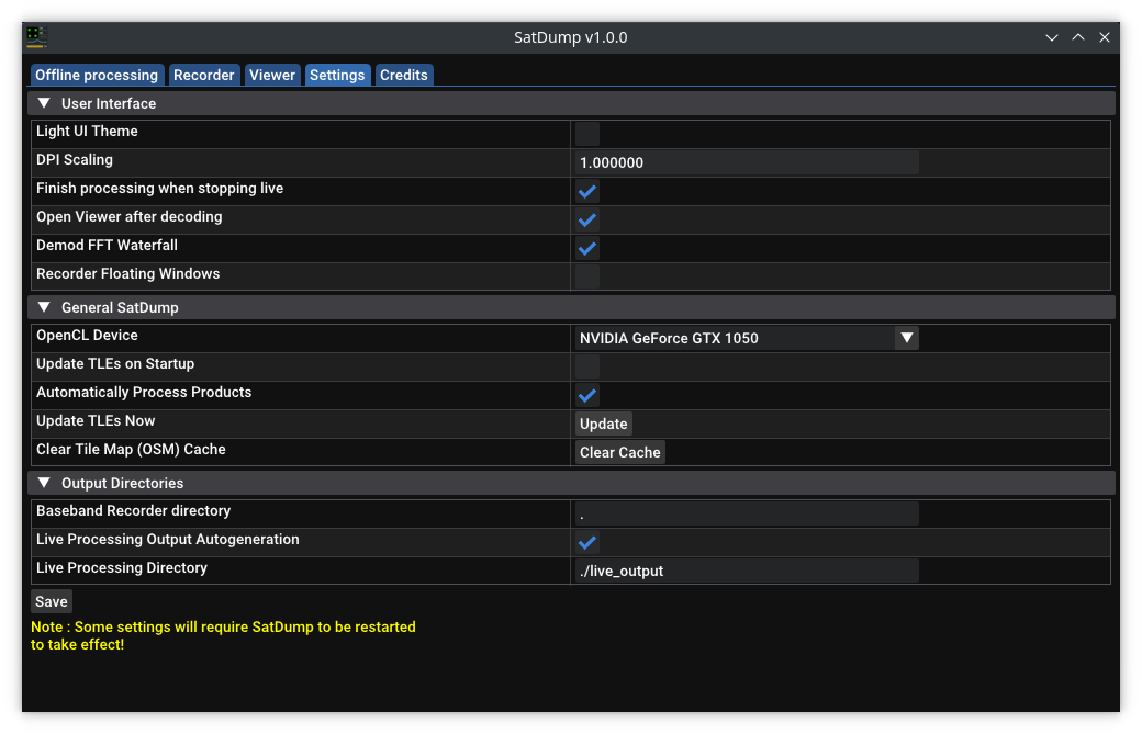
Settings
This is where you can edit the most basic SatDump settings. This section is worth checking out as it contains all the paths and properties!
CLI (this part was made by Aang23)
The Command-Line Interface (CLI) was also entirely reworked, and some major new features were added… That also clearly did cause some confusion so I thought it was also better to cover it here!
First advice : forget how it used to work!
So, first of all now everything is handled through the main satdump command, which comprises 3 modes.
Offline Processing
Just like in the UI, this mode assumes you already have a file to process. The general usage is :
1
satdump pipeline_name input_level input_file.xxx path/to/output_directory [options / parameters]
pipeline_name: Pipeline ID, as displayed when SatDump loads or in pipelines files (pipelines/*.json files)input_level: Input level. This can bebaseband,cadu,frm,soft, or evenproductsdepending on the input file. If providing a baseband that is not WAV / ZIQ, you will need to specify the format and samplerate manually with parametersinput_file.xxx: The input file. Either a baseband, demodulated symbols or frames (Or processed products, providing the dataset.json)path/to/output_directory: Directory where SatDump should write all processed/decoded files
As for parameters, they can in reality be anything you see set in pipelines .json files. But usually, you will not need to change them manually. Though, some demodulator parameters may need to be set manually in many cases :
samplerate: If providing a baseband file, the samplerate of the input baseband file, in Samples Per Second (SPS) or Hzbaseband_format: If providing a baseband file, the baseband format, which can be :f32: 32-bits IEEE Floatss16: 16-bits signed integers (used in 16-bits WAV files)s8: 8-bits signed integersu8: 8-bits unsigned integers (used by 8-bits WAV files)ziq: Custom ZIQ Baseband format, supporting ZSTD compression
dc_block: If your SDR has a carrier at DC due to I/Q Imbalance (eg, HackRF) messing up the demodulator, this should be enabledfreq_shift: Usually this should NOT be required, but it allows shfiting the baseband in frequency in case the recorded signal is not at DC (center)iq_swap: If your file has I & Q inverted. This will happen if using a downconverter with a “High” LO, that is, above the received frequency
And for a few real-world examples :
satdump metop_ahrpt baseband MetOp_Baseband.wav decoded_data/metop_baseband
Decodes a MetOp AHRPT baseband. As the baseband is in WAV format, the samplerate and format will automatically be read from the headersatdump elektro_lrit baseband elektro_l3_lrit.s16 decoded_data/l3_lrit_baseband --samplerate 3e6 --baseband_format s16
Decodes the provided ELEKTRO-L3 LRIT Baseband recorded in s16 format at 3MSPSsatdump npp_hrd cadu old_data/jpss1_data.cadu decoded_data/jpss1_hrd_data
Decode instruments from an already decoded .cadu file. No other parameter is required
Baseband Recording
While before baseband recording was in a separate tool, that is not the case anymore. Instead :
satdump record output_baseband_name --source src_name --samplerate device_samplerate --frequency device_frequency --baseband_format format [others parameters]
record: Indicates SatDump you want to use the recording mode.output_baseband_name: The output baseband name, without the extension. The extension will be set depending on the baseband format you set.
For parameters, you will at least need the following :
source: Source to use, egsdrplay,airspy,rtlsdr, etcsamplerate: Samplerate to record at, in SPS or Hzfrequency: Frequency to tune the device at, in Hzbaseband_format: Same as for offline processing, with a few differencesw16: To record in .wav format (s16, 16-bits)ziq: This default to 8-bits. If you want to use another depth, you can add--bit_depth 16(can be 8, 16, or 32)
timeout: Entirely optional, but sets for how long, in seconds, SatDump should record for
Additionally, you will need to specify parameters for your specific SDR Device. A list can be found here on GitHub.
Live Processing
Normal Use
Live processing is not done through the ingestor as it used to be done. Instead it is done in a very similar way to the recorder and offline processing.
1
satdump live pipeline_name path/to/output_directory --source src_name --samplerate device_samplerate --frequency device_frequency [options / parameters]
As you may see, no input level has to be set, as it will always be baseband. See above for a detailled description of every option. The timeout feature is also available.
Additionally, live-processing in CLI mode can provide current status over HTTP. To do so, you need to set --http_server 0.0.0.0:port (eg, --http_server 0.0.0.0:8080). Once started, you will be able to access a http server providing the live state of the demodulator and decoder(s). That can useful for 24/7 setups where contant monitoring may be required.
For example, on GOES-R HRIT :
1
satdump live goes_hrit output_test_wtf --source rtlsdr --samplerate 2.4e6 --frequency 1694.1e6 --gain 40 --http_server 0.0.0.0:8080
Running curl https://0.0.0.0:8080 will show the following, which can be fed into Grafana or other similar tools for monitoring.
1
2
3
4
5
6
7
8
9
10
11
12
13
{
    "ccsds_conv_r2_concat_decoder": {
        "deframer_lock": false,
        "rs_avg": 0,
        "viterbi_ber": 0.169677734375,
        "viterbi_lock": 1
    },
    "psk_demod": {
        "freq": 1096.974853515625,
        "peak_snr": 2.214721202850342,
        "snr": 0.1323898881673813
    }
}
Server/Client - Network streaming
Another pretty requested features was the ability to only perform some of the steps locally, and forward to another SatDump instance(s) over the network. Perhaps to have a computer near your antenna decoding down to frames (CADUs for example) and another inside processing imagery. This is mostly intended for 24/7 Geo setups (LRIT, HRIT, GRB, HimawariCast, etc).
The “server” is what would run on the side demodulating from an SDR, and the client what receives the data and finishes processing.
Do note that NOT all pipelines are currently supported in this mode. If you wish for one to be added, please open an issue on Github and it will be added.
Otherwise, starting the server-side is done in the same way as live processing and all flags still apply, except you will need to add the following flags :
server_adress: Adress to bind to. Usually 0.0.0.0 is fineserver_port: Port to bind to. You can use whatever you want!
Example for GOES-R GRB (with the http status server as well) :
1
satdump live goes_grb goes_grb_live_test --source bladerf --frequency 1686.6e6 --general_gain 28 --dc_block --samplerate 14e6 --server_address 0.0.0.0 --server_port 5004 --http_server 0.0.0.0:8081
The client will also be started in a very similar way, except of course all SDR-related parameters can be omitted. The client flag has to be passed alongside the server_address (with the IP address of the machine running the server) and server_port. Multiple clients can be connecting to the same server at the same time.
Example :
1
./satdump live goes_grb goes_grb_live_test_client --server_address 192.168.1.54 --server_port 5004 --client